This tutorial draws on some of the online Galaxy tutorials (here) and videos (here) but I have made some of the steps more explicit for you with screenshots.

Galaxy data formats

You can think of Galaxy’s data formats in a few main categories:

1. Sequence data (FASTA, FASTQ)
2. Alignments (BLAST results, SAM and BAM files)
3. Track data (genomic intervals, WIG files — continuous value tracks)
4. Tabular data (many kinds — interval data is a subset)

The key thing is, though, if your data is not in one of the accepted formats you will not be able to proceed. There’s no winging it with data that’s slightly off. If you import a FASTQ file, before you can do anything else, you have to “groom” it into one particular FASTQ format, etc.

Basics of handling NGS data (Illumina example)

First, click on the cog icon at the top of the Galaxy history panel and create a new history. I named mine CMCP6-DE. That history will contain only the files relevant to this exercise so you don’t have to scroll through your old history.

Getting reference genome data

The Galaxy tutorial on this is a little weak. It goes through the mechanics of loading a FASTA file, but it doesn’t make entirely clear what you have to do to have complete information for your reference genome.

You’ll need a FASTA nucleotide file as well as a GFF format file containing the genomic annotations.  Galaxy won’t allow you to load GenBank sequence files, which carry the annotation information along with the sequence. It will only allow bare FASTA files and you have to make a special tweak to the standard header line to get them to work properly.  However, some of the specific pipelines (like the Tuxedo pipeline) that you can use in Galaxy will allow you to add a GFF format annotation file, and you can also visualize GFFs in Trackster.

To get both a FASTA nucleotide file and a GFF file for your genome, go to:

ftp://ftp.ncbi.nih.gov/genomes/Bacteria/Vibrio_vulnificus_CMCP6_uid62909/

I am honestly not sure if getting the data this particular way can be done with the Entrez URL API. The directory names on the FTP site look too nonstandard.  You can always try to figure that out in your copious spare time. Dr. Torsten Seemann goes into the full details of how these directories are organized here. When we pulled down the FASTA sequences of this genome before, we used the INSDC identifiers and used curl or wget to retrieve them from NCBI and EMBL.  Here, files are labeled with their RefSeq identifiers, which map uniquely to INSDC identifiers. The two chromosomes are RefSeqs NC_004459.3 and NC_004460.2.  In the directory above, you’ll see all types of files for each of these two RefSeqs — their annotations from Prodigal and Glimmer, tabular format files, and of course the sequences you need.  Get the ones with file extensions *.fna (FASTA nucleotide) and*.gff (Gene feature format).

Create a “custom build”

You need to make a small edit in your FASTA files before uploading them and this is much easier done with vi than in Galaxy. The current header line in your fresh-from-Genbank genome file will look something like this:

>gi|544163592|ref|NC_004459.3| Vibrio vulnificus genome, Chromosome 1

Galaxy needs it to look like this. With exactly no leading or trailing spaces.

>NC_004459.3

Once the top line is fixed in each of your FASTA files, you need to concatenate your two chromosomes into a multi-fasta file.  Use the cat command in UNIX to do this.

cat NC_004459.3.fna NC_004460.2,fna > CMCP6.multi.fasta

Load only the *.multi.fasta file into your Galaxy.

Next, go up to the User tab at the top of your Galaxy and select “Custom Builds”.  Create a custom build for Vibrio vulnificus CMCP6.

Then load the *.gff file into your Galaxy. Be sure to select your newly created Custom Build as the genome to associate this data with. Select the custom build as your genome for everything you upload for the rest of this exercise, in fact. Now you can visualize your data attached to the genome in a linear browser view using Galaxy’s Trackster, or treat it as a table in the Galaxy analysis interface.

Visualize your data

Once you have your custom build set up, you can use the Trackster application to visualize your results. Trackster is not in the Galaxy tool menu at the left. Instead, it’s accessed in the Visualization tab at the top. It’s a zoomable linear visualization that allows you to see datasets from your history mapped onto your genome, as long as they are in the correct format to be visualized, and as long as you set them up correctly to be attached to your custom build.  Right now all you’ve got to visualize is the GFF file that goes along with your genome.

Click ‘Visualization’ in the top bar to get a New Visualization. Name it something sensible:

Then choose the data you want to load along with your genome:

The result will look something like this, although obviously this particular screenshot is the chloroplast data:

Load the transcriptome data

There are four Vibrio vulnificus CMCP6 samples, two replicates each of transcriptome from samples in artificial seawater, and samples in human serum.  I have pre-processed the  data in two ways.  I trimmed with Trimmomatic, (which creates separate files for paired and unpaired reads; those filenames are inherited in subsequent analyses).

Then, in directory seqtk, there are files from sampling 20% of the original data set randomly. These files are appropriate to analyze using differential expression analysis methods, as if they were a full-sized data set.

In directory diginorm, there are files from single-pass digital normalization of the data. These files are appropriate to use for transcriptome assembly and mapping for transcript discovery.

In this tutorial we’ll use the reduced files generated by seqtk.  Because these files are still pretty large, you need to transfer them to Galaxy by a method other than direct file upload. You can use FileZilla to FTP files to the Galaxy server (as described on the Galaxy Get Data/Upload File from your computer page). Once you load the reads, the first thing that you have to do to every file is run FastQ Groomer.

Load all of the datasets to your Galaxy at once by clicking the checkboxes on the upload page, which will automatically detect the files you have recently uploaded. Make sure you connect them to your CMCP6 custom genome build.

Groom the data

All data must be converted from whatever FASTQ format it’s in to Galaxy’s favorite FASTQ format (Sanger) before any of the other tools can be used.  Use FASTQ Groomer to do this. You’re going to have to run it on each one of the fastq files in your history. Try out the sequence of events for for one file first — run the groomer on it, then run FastQC.

Check the quality

You can use FastQC from within Galaxy to see a report for each of your datasets.  The FastQC output feeds into graphics, and doesn’t feed into downstream processes, so this is sort of a branch of your implied workflow.

 

When you open the HTML file created at the FastQC step you’ll see the familiar FastQC report.

Make a simple workflow

To make this annoying procedure into a workflow, you need to switch to the workflow panel. You did a little bit with capturing a workflow and turning it into history in Galaxy 101. This time you are going to make a workflow from scratch — one that will operate on multiple files in a list.

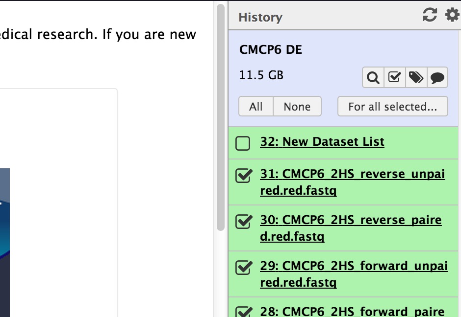
Before switching to the workflow panel, create a new file list.  Click the checkbox at the top of your history to do an operation on multiple files.  Checkboxes will appear at the side of all the items in your history.  Check only the checkboxes on the batch of fastq files that you just imported.

Then click “For All Selected” and choose the option to create a file list. For the operation we’re going to do (running Groomer and FastQC) each of the files can be created separately. We don’t have to pair them. You’ll get a new object in your history — a list. Annoyingly, you can’t rename it. This feature is still in development though.

Then go into the workflow panel and create a small workflow. You need to collect an input list, groom your data, and send it to FastQC.  So you’ll have three items in your basic workflow. When you start with a collection of data as input, your workflow connectors (noodles) will be multiples automatically, and in the workflow boxes you’ll see “run in parallel over all items”.

Next run the workflow. On your input options page you’ll be asked to select a file list rather than individual files.

And you will get back multiple outputs when the run completes.  This can rapidly get messy, because as you’ll see, your output files just refer back to the numbered items in your Galaxy history. They don’t refer back to the informative filenames that were originally uploaded. You can configure to avoid this problem by using the renaming tools at each workflow step.  To do this in an informative way, you need to rename your files using combinations of internal Galaxy variable names (a feature that is apparently documented only by answers to user questions in forum posts at the moment) OR go back and rename items in your history after the workflow completes with the help of the item information in the history.

Trim

Normally you’d insert a trim step here, but you’re working on data that I’ve previously trimmed with Trimmomatic, so you can skip it this time around.

Map

The next steps is to map the data.  The standard pipeline in Galaxy for expression analysis is the Tuxedo pipeline — mapping with TopHat, transcript construction with CuffLinks, transcript analysis with CuffCompare, and differential expression with CuffDiff. This pipeline is a little overpowered for our bacterial gene expression data, because it’s geared to understanding complex transcripts, but since we can’t upload a different set of tools (we use Bowtie, featurecounts, and EdgeR for similar tasks) we will make do and see what kind of information we can get from Tuxedo. It just won’t produce any splice junction information.

Remember, each sample (1HS, 2HS, 1ASW and 2ASW) has four FASTQ files — Ideally, here’s what we want to accomplish for each of the samples:

1. map paired reads
2. map each set of unpaired reads
3. merge all mappings belonging to the same sample
4. construct transcripts
5. analyze transcripts
6. compare differential expression

However, the Galaxy server is a busy place and this may take a while to run. So, if you want to reduce your problem space a little bit, here’s what you should minimally try to accomplish:

for just two of the samples (say, 1ASW and 1HS):

• map paired reads only
• construct transcripts
• analyze transcripts
• compare differential expression

TopHat

TopHat runs on your reads and produces, among other things, a BAM file (binary alignment).  There are a TON of input parameters, and you are not likely to get them right or to get the best results without digging into them and trying to understand them.  For demonstration purposes you can run mostly with the default parameters, although we know for sure the insert size for this read set is 400 and the standard deviation is 35.

Your BAM file can also be converted into BAI and BigWig formats, and it can be displayed in Trackster along with the GFF annotations, so as a result you see where individual reads map.

CuffLinks

CuffLinks is going to take that BAM file and try to create transcripts out of it as well as calculating FPKM (fragments per kilobase per million reads) which is a normalized measurement of expression level.

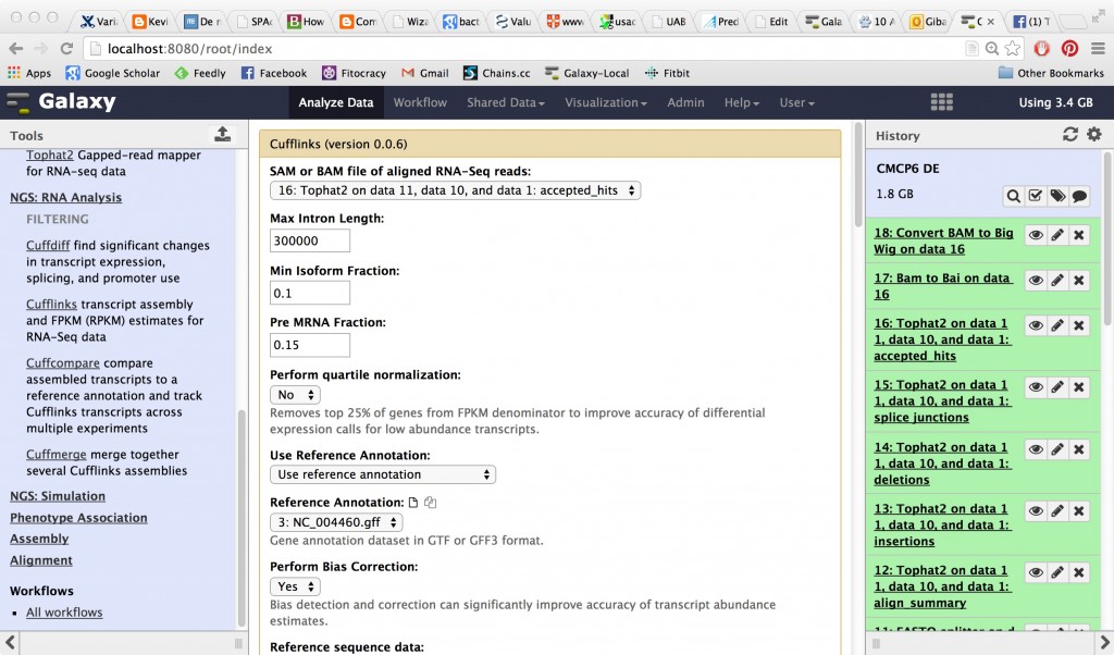
CuffLinks will have several outputs, including a tabular gene expression file:

And assembled transcripts that you can compare to the existing annotations on your genome, in Trackster. You could also use the table manipulation tools (which we briefly saw in Galaxy 101) to make comparisons between these files.

The last two steps you should be able to figure out how to execute based on your familiarity with the RNA-Seq analysis process from CLC and other contexts, but if not, no worries, we’ll discuss them.

CuffCompare

Works on your assembled transcriptome and compares it to the reference annotation.

CuffDiff

Works on your  gene expression values and produces an analysis of differential expression. Notice that you need to set up two (or more) conditions and connect your samples to the correct condition.